
How do I get my team to capture daily metrics without extra friction?
The eternal struggle in a leader’s life – and when working without proper tools – is data collection. Some call it the manual tracker, some call it “a lot of work for me”, others probably just accept it as part of the issues they just need to deal with, and others try to find new and interesting ways to make it go away… or at least mitigate some of the effort.
The truth is very scary for people because around 54% of businesses use Excel as the core operational tool and 75% of companies (a recurring number industry analytics keeps providing) still rely on manual logs, spreadsheets, paper, and other similar methods. Decades of digital evolution, tons of posts and discussions on the topic, and advice about how to embrace the digital and move away from the “ol’ fashion” – and here we still are, ol’ fashion and all.
With the ever-growing pressure on data, the increase in AI adoption (that also needs reliable and stable data to provide valuable outputs), and the constant distancing from traditional approaches, using unreliable or very difficult-to-manage data collection workflows is honestly a nightmare. It is true that many of us are not in a position to change company-wide procedures or force them to invest in more accurate or up-to-date tools or systems, but we can, however, find the best solution for now. Investing a bit of time and effort into this will save you hundreds of hours later on.
What do I need to know or do to have better data collection with the tools I have?
To fix your data collection using only Excel, start by using Data Validation to add drop-down menus and stop messy manual entries. Next, use VLOOKUP with IFERROR to auto-populate targets effortlessly. Finally, build individual and team views with SUMIFS and AVERAGEIFS formulas to track performance transparently, saving you hundreds of hours of headache.
In this article:
- The current reality and struggles: Manual data entry causes team frustration, unreliability, and fake information, forcing leaders to rely on cumbersome trackers.
- Start with the basics: Establish a structured baseline by auditing what you need to track and utilizing Excel Data Validation drop-downs to prevent erroneous entries.
- Building the workflow: Automate repetitive data entry by implementing VLOOKUP and IFERROR formulas to pull target information cleanly without manual typing.
- Crafting better overviews: Build dedicated individual and team performance views using SUMIFS and AVERAGEIFS formulas to provide complete operational transparency.
- Closing thoughts: Putting a few hours of upfront effort into building a simple, semi-automated tracker saves hundreds of hours of headaches and protects your mental health.
The current reality and struggles
At this point, new or experienced manager, everyone knows that any type of manual data entry will break the team. It’s tedious, it’s hard to track, a complete nightmare to correct, and almost never truly accurate. A lot of effort goes into these activities, with them the added pressure, the bad leader-to-team communication, the constant reminders and discussions, the negative employee experience – not to mention the reflection in the results or the analytics extracted from that manually added data. On this topic, I found this not-so-fun fact: surveys by project management authorities like Wellingtone indicate that over half of organizations (54%) still do not have access to real-time project KPIs, meaning leadership teams rely on manually compiled status updates, static slide decks, and individual department trackers to understand operational health. Makes you think twice about joining a company, or at least asking them how much manual data entry they have!
Alongside all the above-mentioned pleasantries, we also have a multitude of cause-and-effect aspects, like the fact that clunky spreadsheets lead to fake data. Fake information in turn leads to very bad decision-making, improper measurement, faulty business directions, and is more likely to fail than to succeed. Just think about your basic manual tracker where people just put in all the work they are doing without any actual verification – people can make up different timelines, dates, orders, tickets… whatever you can think of, and if something bad happens or they end up caught in a lie they can always say “I forgot” or “it’s a mistake”. You can’t blame them; in the end, this is not 1920 where people track the work they are doing on a piece of paper.
Your job, as the leader, is to make sure some of the pressure from this perspective is reduced, and the best way to achieve this is by implementing better workflows – even with the limited available tools you might have (say, only an Excel file). The idea is not to create a new-age revolutionary tool, but to use whatever you have to your advantage and find better ways of doing it.
Start with the basics
In your quest to find better ways to collect your data, the first thing you need to do is go back to basics: the current tool you have. Look at what you have right now and try to establish what your process is about, what you need to capture, and how to capture it. If you need a quick refresh on these topics, I suggest you give these two articles a good read: Creating Your Team’s First Charter and Business Process Management Systems (BPMS) Basics. If you are struggling with data as a first-time manager, don’t worry, I got you. Check out these: Intro to Statistics: A First-Time Manager’s Guide, Data Types: A Beginner’s Guide, and of course, I’m Not Good with Data: The Non-Analytical Lead’s Guide.
For the basics, let’s take an example and say we have a small team with different types of metrics we need to track. Sadly for us, the entire tracking must be done manually, so each person goes into a tracker and adds whatever information they need to. Without a proper workflow, this becomes something out of a horror movie, with the leader having to correct, check, and ask at every single click. To avoid going crazy over an Excel file, let’s say we scratch everything and rebuild it from the bottom up. We will assume these are the basic things we must track.

To transform this into a better workflow, we need to list all the items people would normally add here. For example, in the Metric Name, we can have Customer Tickets Resolved, Average Speed of Answer, Hold Time, etc. In the Status, we could have Open, Pending, Closed, etc. Basically, we are creating categories for each single column name and trying to list every possible item people could add there. To avoid strange or erroneous data capture, we can also add a list of numbers (in my example I added from 0 to 100) that can be used to capture the actual numbers (tickets closed, average speed of answer, hold time, etc.). Remember, we are not looking for perfection; we are looking for something quick, efficient, and as accurate as we can make it.
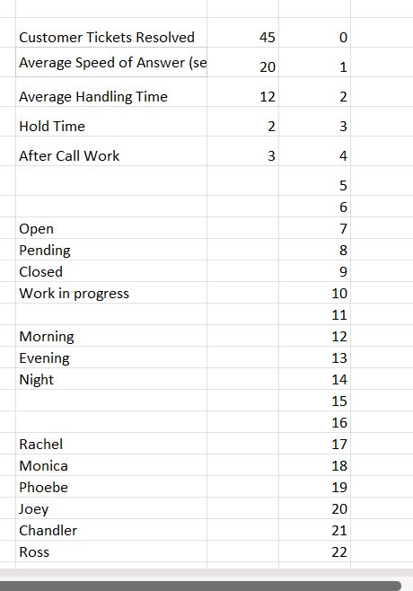
When we have all of this listed, it is time to use one of those Excel features that people sometimes forget about: Data Validation. This option will allow you to insert a drop-down menu for every single cell in your sheet, this way mitigating any potential issues you might get when or if people would add the data manually on their own. It’s not perfect, but it’s better than nothing.
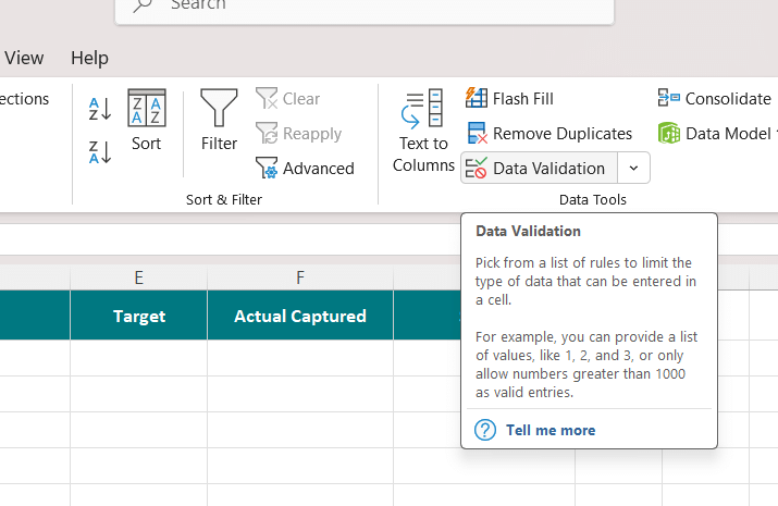
In it, you have plenty of options for all sorts of things: whole numbers, decimals, list, date, time, etc. Usually, you would select list, but feel free to play around with it and make the best use you can of it.
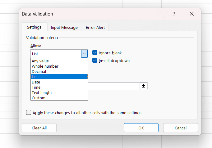
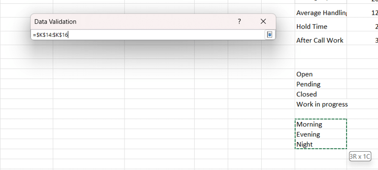
In my example, I start by adding the type of shift (Morning, Evening, and Night). It would look like this:
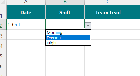
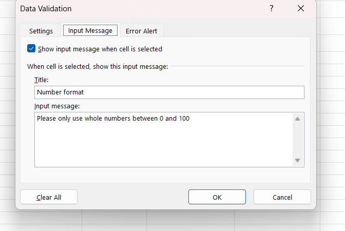
You can also add an input message that will appear each time someone is trying to add something in that field.
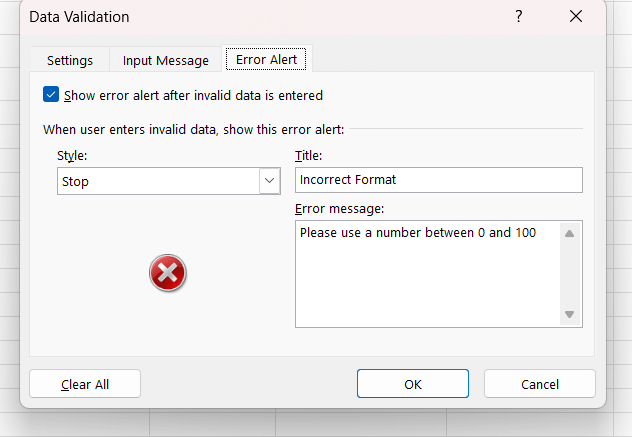
And if you want to go the extra mile, you can add an error alert type of message that will appear each time someone is trying to bypass the drop-down by typing in the cell something not included in the list. Note however that in normal Excel files you can bypass this by copy-pasting over the cells; however, this option can be turned off if you protect the sheet and people will no longer be able to copy-paste over, but will be able to use the drop-down.
Building the workflow
With the basics done, it is now time to look ahead and think about other ways to minimize the effort people are putting into this tracker. A good question to ask here is: what else can I do to cut the time needed to fill in this file?
In my example, I started using VLOOKUP to get some of the data, like the targets. Why should people add them manually (or even in the drop-down) every single time when a formula can do that for us?
If you never used it before, here is how you do it. Start with the actual formula (VLOOKUP).
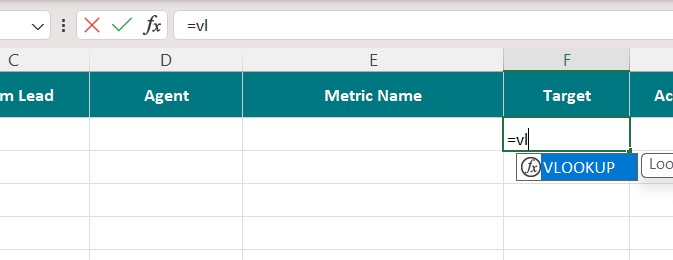
The first thing you need to put in is the lookup value, meaning what exactly are you trying to find. Think of this formula as a search function: you tell it what to search for and where to find it, and it will do the work for you.
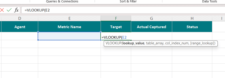
Let’s say I want to have the target information auto-populated based on the metric name. I have a small table with each metric name and the associated target on the right side (this will be the “place” where the formula will search for the info needed). In your case, the value we need will be in the column Metric Name, so just select the first cell in that column (not the entire column or the header, just the first value). In my example, because there is a drop-down in it, you don’t have (yet) any actual value selected there, but that is fine.
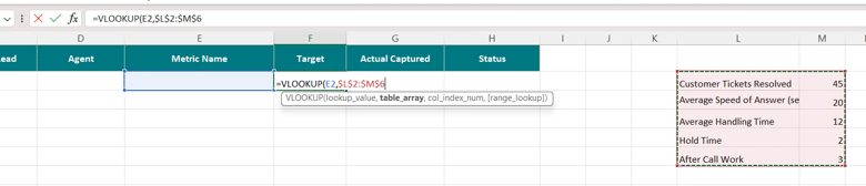
Then we need to give it the “place to search for”, also called a table array. In my example, I just selected the entire table on the right side. Mention here: when you have a similar example with a smaller table to search in, you must lock the table in. You do this by using either F4 or Fn+F4 on your keyboard (depending on your PC or laptop – and I’m not sure for Apple as I don’t use it). You know it is blocked once the table array is surrounded by dollar signs. This means that when you drag the formula down, it will not drag the table as well.
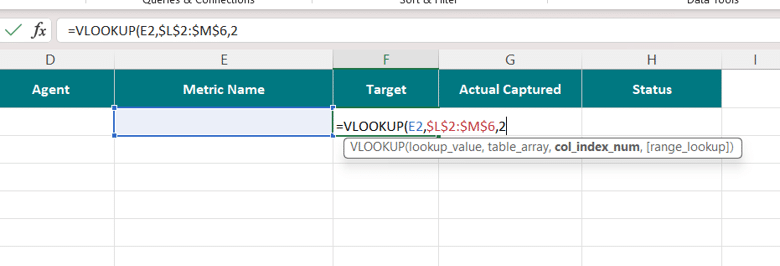
Next, it’s time to indicate the column number you want the formula to return. In our example, we have a table with two columns: one with the metric name and another with the target. Since we are interested in the target, the column we need to add is number 2, so you just need to put “2” in your formula.
Finally, we have TRUE or FALSE, meaning an approximate match or an exact match. We are interested in an exact match, and as such, we will put in FALSE.

If you managed this far, you should have the lovely N/A (well, if you used my example anyway).
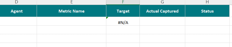
Because we don’t have any actual data in Metric Name, the formula will return N/A, meaning it is not finding anything. If you want to go the extra mile and remove all the N/As from your file, you can use a simple trick: IFERROR. This formula is added just before the actual VLOOKUP and will hide any errors the formula gives. All you need to do is add it right after the = sign, put a “,” after the VLOOKUP, and then in “” just put whatever you want to see instead of the N/A. I just left it like this “”, meaning I don’t want to see anything.
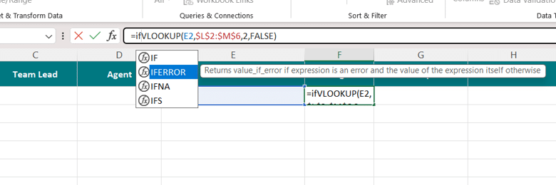
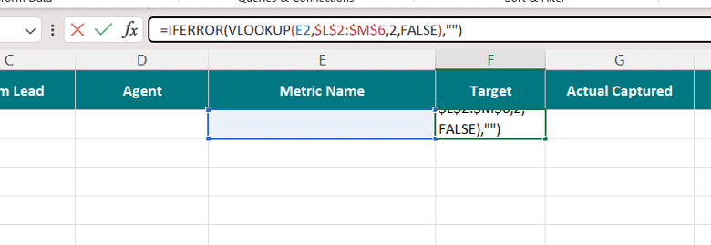
And the final result, with one metric name selected and the rest not selected, should look like this.
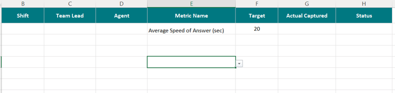
As you can see, the sheet is already looking better and much more efficient than whatever was there before.
Crafting better overviews
A very common problem I have observed across time is people not having enough visibility on what they are doing. Because I am a firm believer in transparency, I try the best I can to offer this to people. When people know where they are and where they need to go, things are much easier. How can someone improve on a metric if they can’t see what they did? And no, it is not the obligation of the employee to monitor their workload; that is the leader’s job (it’s in the name after all, isn’t it?)
A simple thing like a manual tracker, with a bit of effort, can become a very powerful tool for both you and the team, so let’s see how we can make this happen. Any good database will offer, alongside a better way of data collection, different options to track both individual and team performance. On any tracker you might have that stores data on performance, I strongly recommend two additional views: the individual view (where you can see all the people in your team and how they are doing per metric) and the team view (with the overall performance of the team).
Individual View
In my example, it would look something like this:
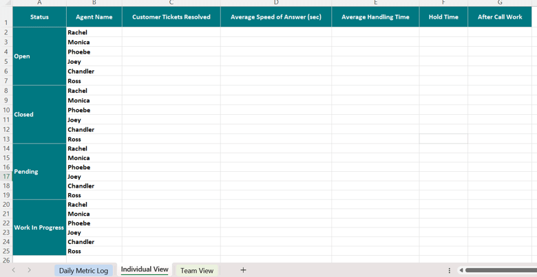
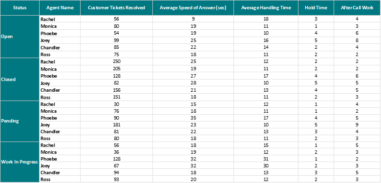
My idea here is to bring each of the metrics collected in the first sheet to this one, but on an agent and status level, meaning what each agent did on each metric per status (open, closed, pending, and work in progress). This way, everything is here in the open for everyone.
To achieve this, we will be using a series of formulas, mostly SUMIFS and AVERAGEIFS. They might appear complicated, but trust me, with a bit of practice, you will be an expert in a few minutes. They all follow the exact same formula structure; the only thing that is different is the function: one will return the SUM and the other the Average.
First thing is the formula, like so:
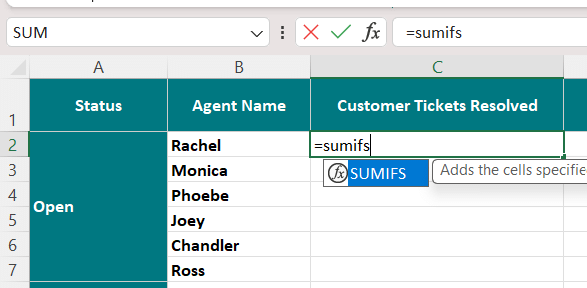
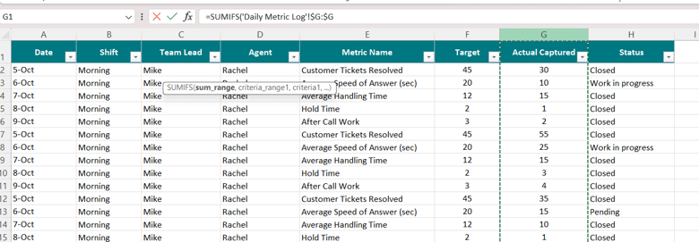
The first and most important thing to add is the range you want to measure. In my example, the only column that has data I can actually use for calculations would be column G (where people fill in the data), so this will serve as the sum range. After this, you just need to repeat the following: criteria range (the place where the formula must check the criteria used) and the actual criteria. In my example, to find what Rachel did with Customer Tickets Resolved for Open status, I must select three criteria: the metric name (range is the column with the metric name and criteria name “Customer Tickets Resolved”), the agent (range is the column with the agent name, while criteria is “Rachel”), and finally the status (range is the column with the status and the criteria is “Open”).
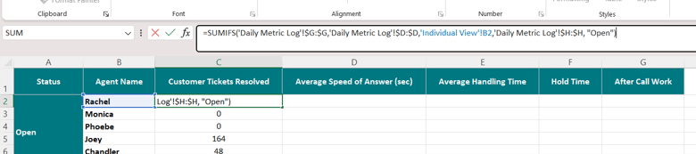
Once you have added all your formulas, you should get a lovely sheet with auto-populated data based on the first sheet. This will serve as your main source of team results, where you can quickly check what each person is doing, where you might have issues, etc.
Team View
This is all about the entire team. Your responsibility, as the leader, is this specific sheet. In it, you have the overall view of how your team is performing and what areas are doing well or need improvement. Without a team view, you as the leader are not actually managing. Using the exact same formulas, but adapted for this sheet, you are able to create a much more condensed view with all the information you need.

Closing thoughts
What I have shared today is only one way of doing this. Excel offers a wide range of methods one can use to achieve the same result, and as more articles are released, I will present other methods. For now, I focused on building something using simple formulas that don’t really require a very complex understanding of Excel. Plus, in the current era, you can always pop your file into whatever AI model your company is using and ask it to build it for you, but I prefer the more traditional methods, especially when doing it for the first time. You can’t ask AI to create something you really don’t understand – otherwise that movie becomes a reality (you know what I’m talking about).
Jokes aside, I can’t stress how important and vital having better collection methods for your data is. The lack of them or the complete surrender to the “As Is” is a big No-No for any leader, and for those of you just starting out, put the effort in and make it right from the start. Don’t ruin your experience, time, and mental health with messed-up manual trackers or complicated reports that can easily be semi-automated or improved with just a few hours of work.
Until the next one, stay healthy, happy, and safe!