Excel & Sheets Essential: The 4 Must-Have Tools

Which spreadsheet tools do I actually need to master for reporting?

Life in operations is complex, and for the people manager, the picture is less “standing around and giving orders” and more “working on at least 10 different things at the same time”. In the middle of this messy world, with pressure from both teams and higher management (and at times also customers), it’s no wonder the first and middle management layers are usually the ones with the biggest attrition and are labeled as “hard jobs”.

A major skillset every leader should have is without a doubt data analysis, with your individual capability in “spinning the numbers” actually predicting a big part of your success. The reality is simple: those who know how to manage data are the ones who will survive. In the life of a new leader, there are a few elements from Excel and Sheets that one should master for a better overall experience, like a basic foundation, if you will, in “the things you will be doing a lot”.

Like any other topic, Excel and Sheets is a big topic with many layers to it, and there is always the question of what specifically a first-time manager should know from the start and what possible benefits you get if you know them?

Managing operational chaos starts with taking control of your data. First-time managers need four essentials: LOOKUPs to link datasets, conditional formatting to highlight priorities visually, pivot tables to summarize complex operational information quickly, and basic statistics (SUM, AVERAGE, MEDIAN) to track team outputs. Mastering these core tools saves precious time, eliminates costly errors, and drives confidence in decision-making.

In this article:

The LOOKUPs: VLOOKUP and XLOOKUP automatically connect separate data sources using a unique key, saving you from copying and pasting missing information by hand.
Conditional Formatting: Setting up dynamic color rules highlights key statuses and deadlines automatically without turning your spreadsheets into a chaotic rainbow.
The Pivot Table: Pivot tables effortlessly transform large, complex datasets into clean summary tables with just a few clicks.
Quick Team Statistics: Basic formulas like COUNT, SUM, AVERAGE, and MEDIAN make calculating team performance straightforward and stress-free.

The LOOKUPs

Many of the struggles that we have when dealing with a lot of data come from trying to put together multiple data sources, add missing information, correct things, import others, and so on. For this exact reason, we have a dedicated family of formulas in Excel that are created specifically for this type of work: LOOKUP.

The primary idea behind these functions is very simple: you look up something you need in another file using (what is normally called) a primary key. The key is a UNIQUE identifier that is present in both places and will serve as the “link” or search helper to bring whatever missing value you need from one place to another.

We have 2 mostly used LOOKUP functions: VLOOKUP and XLOOKUP, and here are the main points to consider for each.

VLOOKUP – the classic choice for many:

Only looks right: Your lookup value must always be in the very first column on the left of your selected range. It cannot pull data from columns to the left of your search key.
Relies on column numbers: You have to count columns manually (e.g., column 3, column 5). If someone inserts a new column in the middle of your sheet, your formula breaks.
Requires exact match reminder: You must explicitly type FALSE (or 0) at the end of the formula; otherwise, it defaults to an approximate match and returns wrong data.

XLOOKUP – the modern standard:

Looks in any direction: It doesn’t matter where your lookup column or return column is – left, right, up, or down.
No column counting: You simply highlight the search column and the return column separately. Inserting or deleting columns won’t break your formulas.
Built-in error handling: If a value isn’t found, you can specify what text or zero to display right inside the formula instead of wrapping it in a clumsy IFERROR statement.
Exact match by default: It assumes you want an exact match, saving you a keystroke.

In terms of advantages, XLOOKUP is without a doubt the winner, as it is flexible, has exact match by default, has built-in error management, and you no longer need to count columns like crazy. However, not all Excel files might support it, and some older ones will still only have the VLOOKUP variant.

To better understand, let’s take an example and see what they are all about. Say we have the following tables with information:

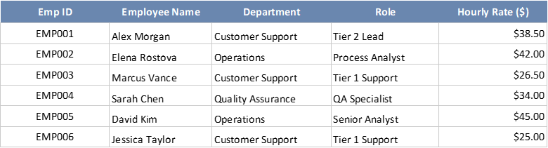
Our second table has some information that we must fill in using different methods (I’ve decided to showcase both of them, just in case). We will need the employee’s name, the department, and based on the hours logged, we need to calculate the total cost associated with each employee in the last column of our 2nd table.

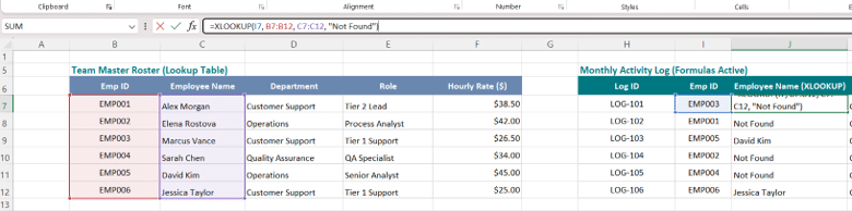
To bring the Employee Name, we will use XLOOKUP. The formula will ask for the following:

Lookup Value: the key; in our case, it will be the employee ID since it is present in both files and is unique
Lookup Array: this is the column where the key is present in the other table (in our case, the Team Master Roster, as we are bringing info from this table to the Monthly Activity Log)
Return Array: this is the column that contains the specific information you need it to return (in our case, the employee’s name)
If not found: what the formula should return for you

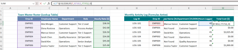
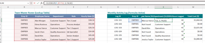
For the Department, we will be using the classic VLOOKUP, which will request from you the following:

Lookup Value: the primary key, the employee ID in our case
Table Array: where specifically the information is located. Note that the formula only works from LEFT to RIGHT, meaning the Key must be the first thing in the table you are searching.
Column Index Number: the number of the column you need it to return (in our example, department is the 3rd column, so we will add the number 3)
Range Lookup: here you have either TRUE (approximate match) or FALSE (exact match). I always use FALSE.

Conditional formatting – the only colors you need in Excel

Think about this one as really great makeup in creature movies: the better you are with it, the better the look of your creature. In data analysis, it’s difficult to see things with the “naked eye” because there are a lot of things around us, so we need a bit of help. This is where conditional formatting comes in and helps.

There are many things one can do with conditional formatting, but I just want to show you the clear, simple, and easy-to-apply aspects that will get you going as a first-time manager (or curious person).

As with many other things I do, we will take an example: say we have the following table that is tracking progress on different aspects: task name, owner, due date, days overdue, status, CSAT score, budget, money spent, and variance between budget and spent. On this type of table, you have 2 possible scenarios:

Manually color things by hand like an old pro and waste a lot of time on something that will need to be redone each time things change
Use conditional formatting, do it once, and be done with it.

Of course, you could also leave the table exactly like this, but honestly, when you add a bit of drama to your data, things look just a bit better. If all tables and dashboards looked like this, we would just give up.

Now, before we begin with this, I have a very special note to add: LESS is MORE, and no one likes a table completely covered with conditional formatting that would maybe look like this:

With that out of the way, let’s start with something simple, elegant, and easy to do: Status. We can have a visual code based on the text it has:

Red for Overdue
Green for Completed
Yellow for In Progress

To achieve this, we need to apply the same rule, but with slightly different aspects, like so:

Select the column you want to beautify
Go to Conditional Formatting – Highlight Cells Rules – Text that Contains
Put in the text and the associated color (red for overdue, for example)

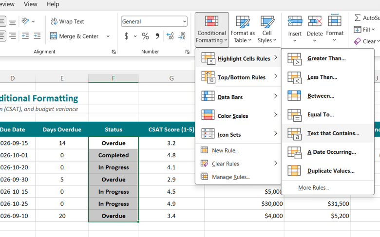
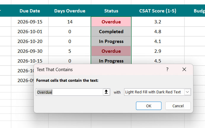
To achieve a 3-color code, just repeat these steps 2 more times, changing the text and color to green for completed and yellow for in progress, and you will get this result:

In the end, I have decided to go with this final look for my table, but you are free to experiment and add, remove, and play around with whatever you want. Try it out and see what works best for you.

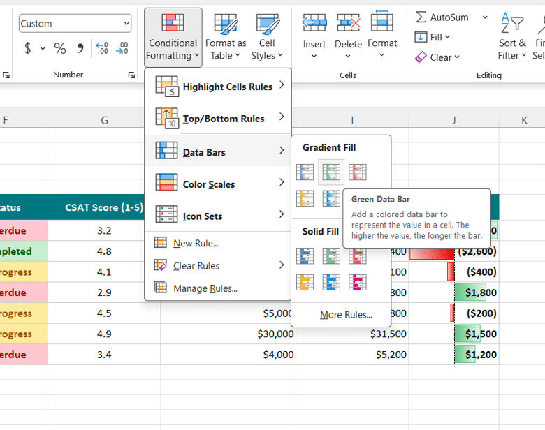
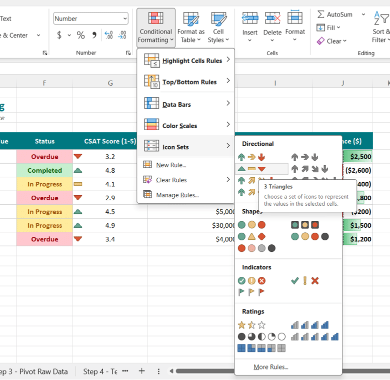
For the other 2 columns, I used the options below, in case you want to see the details. Don’t worry; this is very easy – just select and click.

The Pivot Table – the must-have skill of any Excel user these days

Many years ago, pivot mastering was something else, but today it is one of the most essential and necessary skills someone working in Excel needs to know. There is no way around this topic anymore: you either know it or you must – there’s no more doing the job without using pivot tables. The amount of data and complexity of analytics are no longer manageable with simple tables people can manually create (not to speak at all about the influx of AI capable of data analysis in a few simple clicks).

So, what exactly is a pivot table? For those of you who don’t know it, and to put it very simply, a pivot table is a tool in Excel that will allow you to create a table. Yes, you read that right: it’s a tool capable of transforming any dataset into a table where you decide what to put in.

Let’s see it in practice, and like all other things, we will be using this table as an example: a database with information about tickets, date, lead, category, priority, CSAT, resolution, and status.

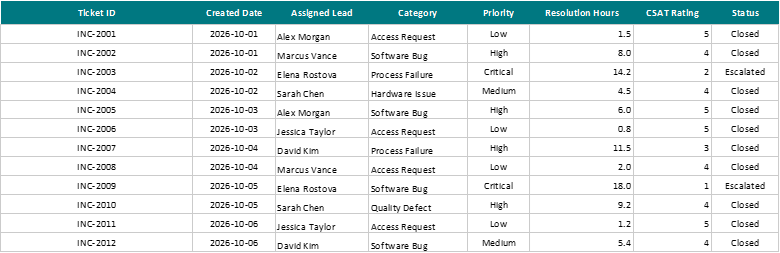
From this, I can extract an entire list of tables with just a few clicks. Let’s assume we need the following aspects:

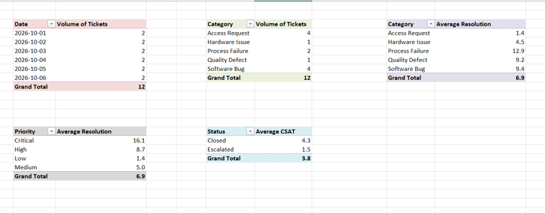
Tickets per Day
Tickets per Category
Category and Average Resolution Hours
Priority and Average Resolution Hours
Status and Average CSAT

Now let’s get to work and make them happen. Just select your dataset and go to Insert – PivotTable, and then click OK.

For the first table, just drag the Date into the Rows, and Ticket ID into Values. Make sure Ticket ID shows up as Count and not Sum, since you need the number of tickets.

For Tickets per Category, you can just copy-paste the entire pivot 2 columns to the right and replace Date with Category.

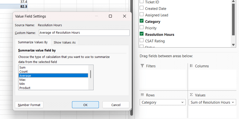
Now just copy the pivot again, and this time replace Ticket ID from Values with Resolution Hours. Initially, the pivot will automatically use SUM for it, and you need to change it by clicking on the little arrow next to SUM of Resolution Hours, clicking Value Field Settings, and selecting Average from the list.

For Priority and Resolution, just replace Category with Priority.

For Status and CSAT, copy the previous pivot and replace Priority with Status and Resolution with CSAT (keeping Average in case it changes back to SUM).

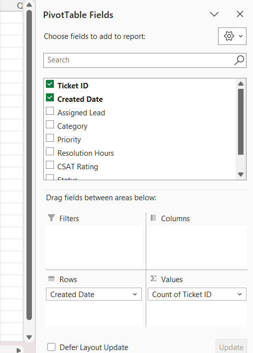
Like any other table, pivots can also be beautified a bit, and you can improve the way they look by updating the names, using different colors or pivot models, etc. In the end, a very simple result that took me 5 minutes max looked something like this:

Quick Team Statistics

Finally, we have arrived at the “crème de la crème,” as they say: the statistics! I know, folks, we just can’t escape this topic. Sadly, it is everywhere, and the faster we embrace it and make peace with it, the better it will be for all of us.

While some of you might be thinking that this will teleport us back to those really bad math experiences we had in school, trust me, Excel makes the experience far less “school-like” and more pleasant and easy to follow and understand.

The basic pack for a first-time manager when it comes to statistics and business would normally cover the following concepts:

COUNT: will count the number of items that appear in a specific place
SUM: will return the sum of a selected data range
AVERAGE: will return the mean or average value of the selected range
MEDIAN: will provide the median value of the selected range
MIN: will provide the smallest value from your range
MAX: will provide the largest value from your range

Let’s use this table as a study example and see what we can do with it. We have a simple table with some people and 5 tickets. Using this as our basis, we will go ahead and calculate different statistics.

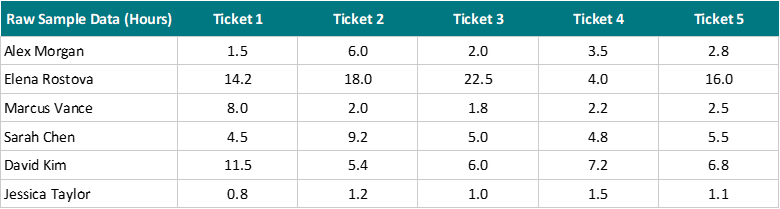
In the end, we can create this table with the team results and individual results based on the original dataset.

Before we close, I would like to provide this list of articles I have already published about this topic. In them, I detailed everything you need to know about data, a statistics intro for the first-time manager, and other essential information you need when starting the job:

Until the next one, stay safe, healthy, and happy!